- MEMS Oscillators → Silicon beam oscillates at a stable resonant frequency (e.g.\ 32.768 kHz).
- Mass Sensors → Resonant frequency shifts when adsorbed mass increases (e.g., molecule binding).
- Resonant Pressure Sensors → Membrane tension changes with pressure, shifting resonance frequency.
- BAW/SAW Filters → Piezoelectric excitation generates acoustic waves with frequency-selective response.
Development of a Full-Field Interferometric System to Detect Low-Frequency Vibrations in Micro-Acoustic Components
Master's thesis conducted at Qualcomm RF360
Topics covered:
Problem Context → Some Preliminary Theory → Measurement System Development → Experimental Validation → Conclusion
MEMS Characterization
Choosing a Measurement Technique
Measurement Requirements
- Operating frequencies mainly below approximately 1 MHz
- Sub-nanometer displacement sensitivity
- Cost-effectiveness and practical usability in a laboratory environment
For dynamic MEMS characterization, optical non-contact techniques are particularly attractive.
Commercial turnkey instuments are availale but custom platforms offer more room for flexibility.
Two techniques stand out:
Scanning Laser Vibrometry
Offers extremely high sensitivity and a very wide frequency range, but typically requires specialized and comparatively complex hardware.
Full-Field Stroboscopic Interferometry
Requires less hardware effort and is better suited to cost-aware laboratory setups, although the per-pixel sensitivity is lower because the available optical power is distributed across many pixels.
Decision
Despite its lower per-pixel sensitivity, modern full-field interferometric systems can still achieve sub-nanometer resolution and are therefore well matched to the requirements of this project.
Wave Interference
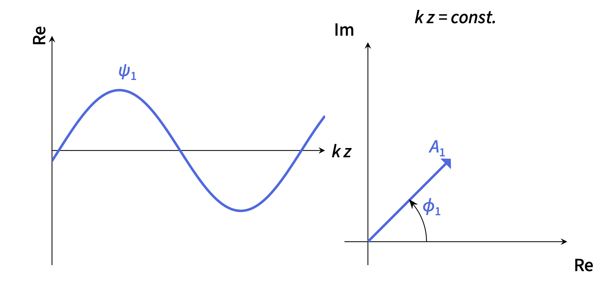
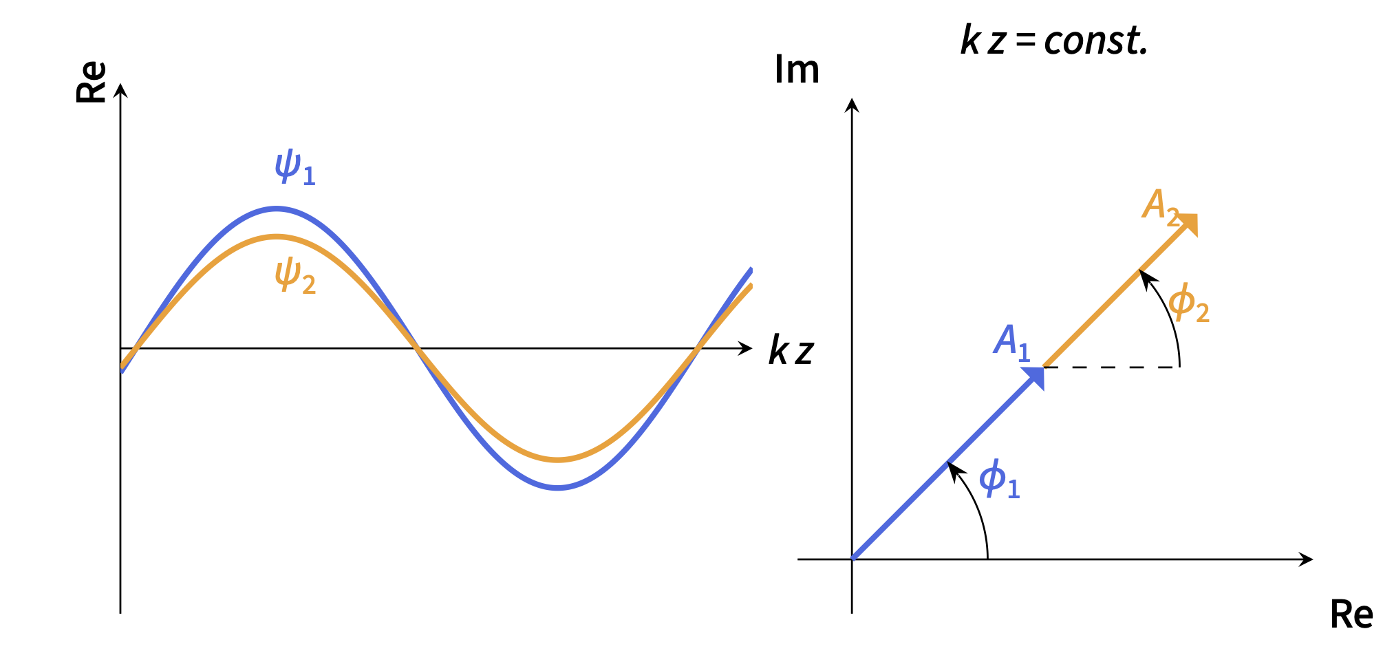
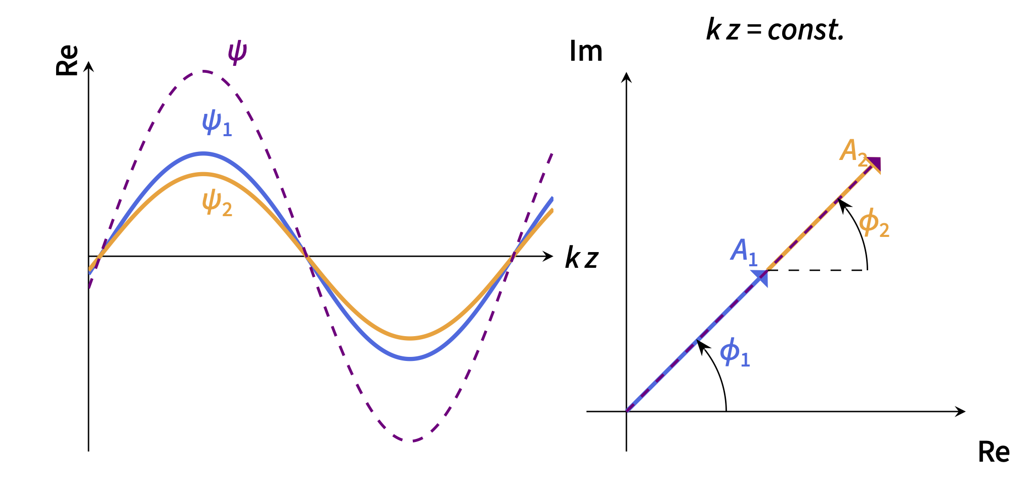
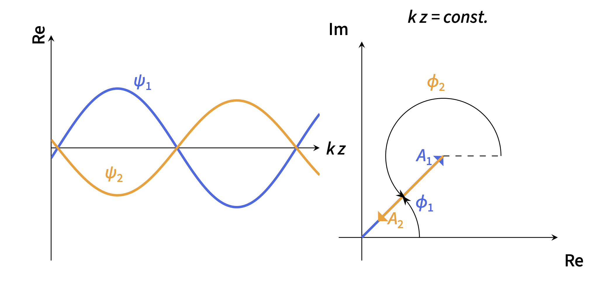
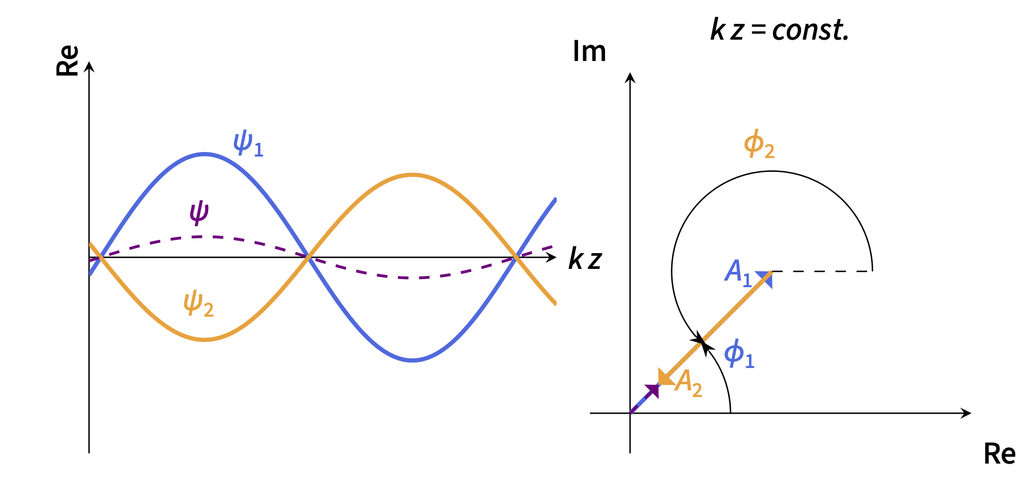
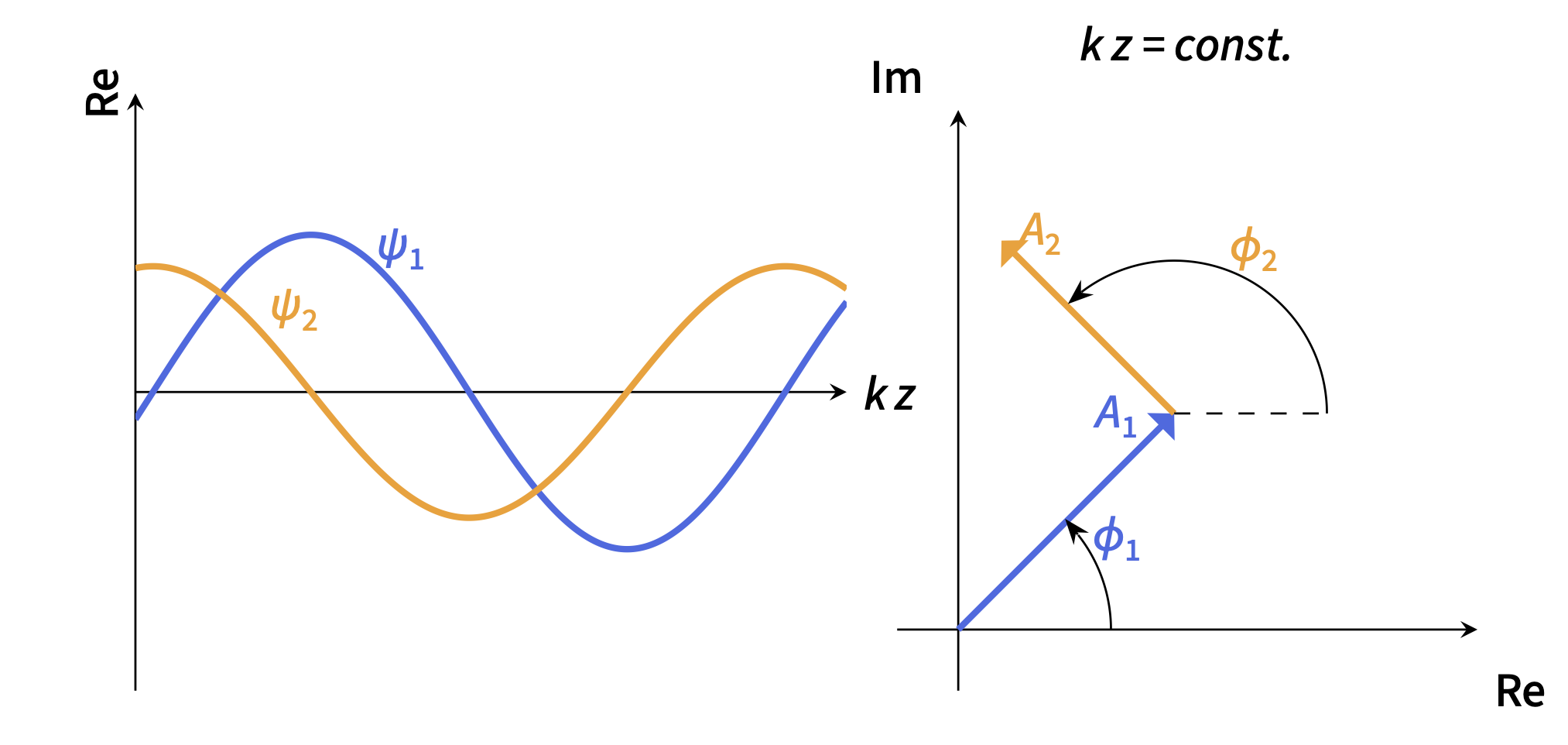
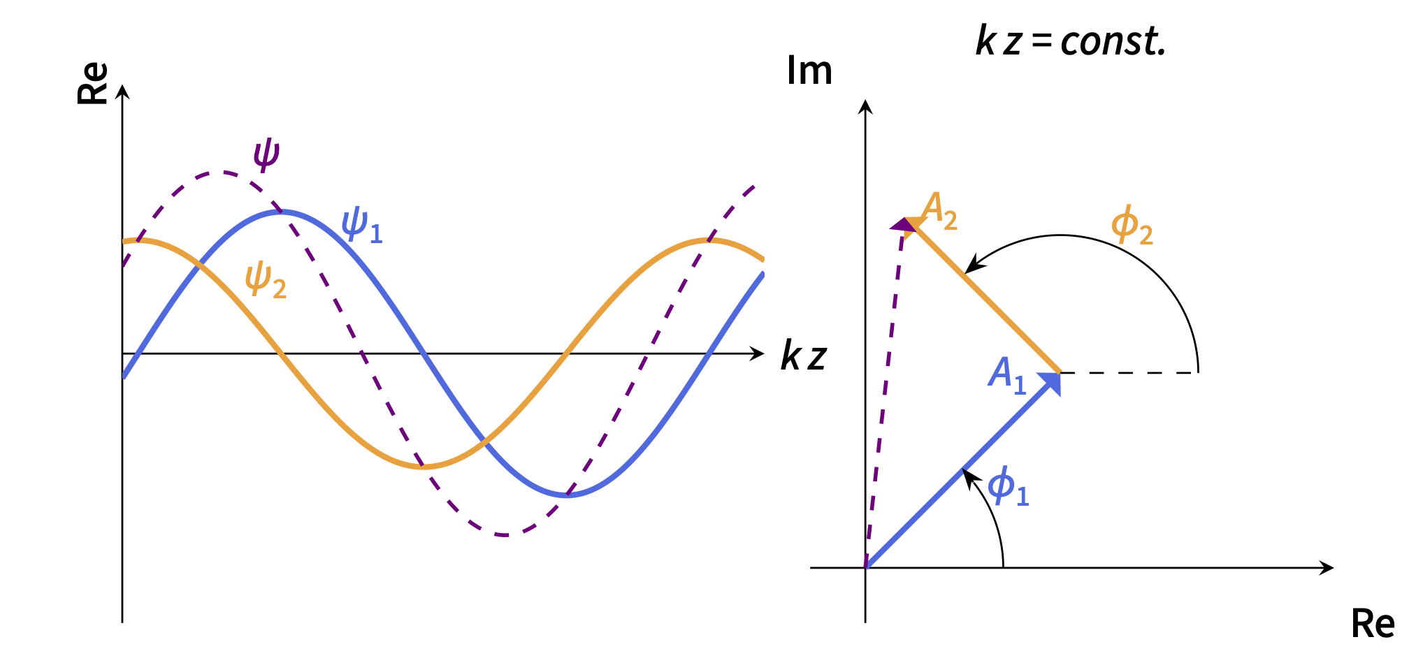
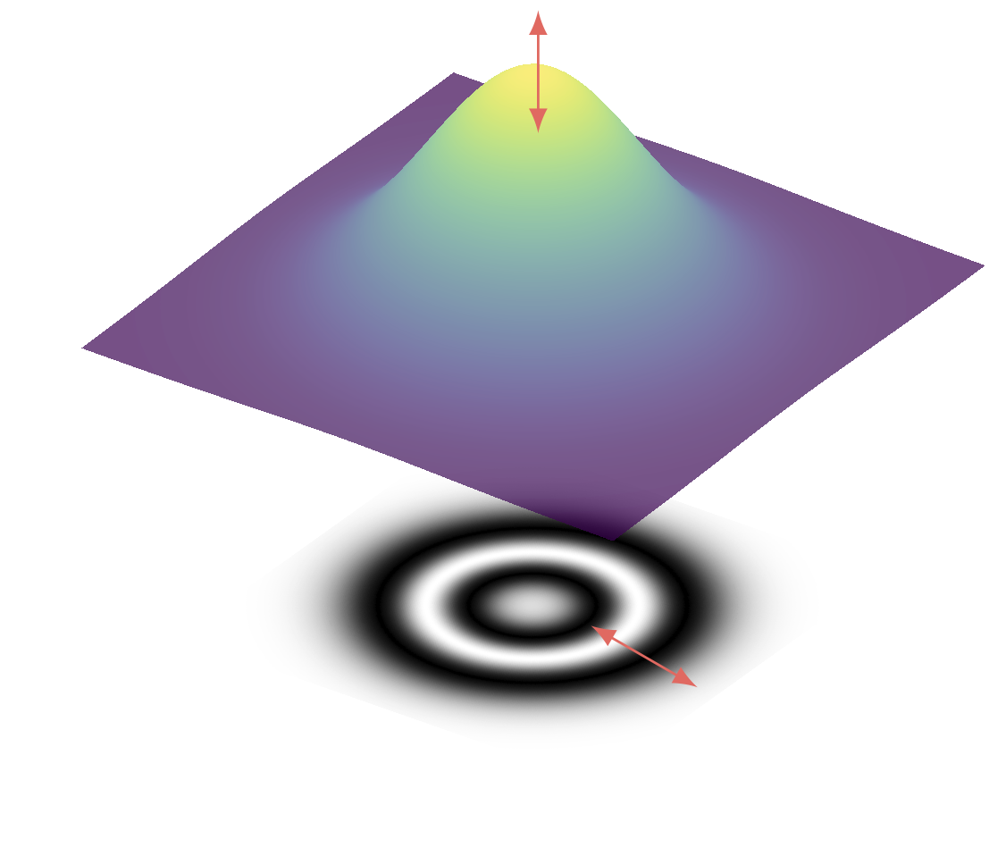
Constructive interference occurs when the phase difference is an integer multiple of \(2\pi\): \[ \Delta\varphi = 2\pi n, \qquad n \in \mathbb{Z}. \]
Destructive interference occurs for odd multiples of \( \pi \): \[ \Delta\varphi = (2n+1)\pi, \qquad n \in \mathbb{Z}. \]
In between, patially constructive/destructive interference occurs.
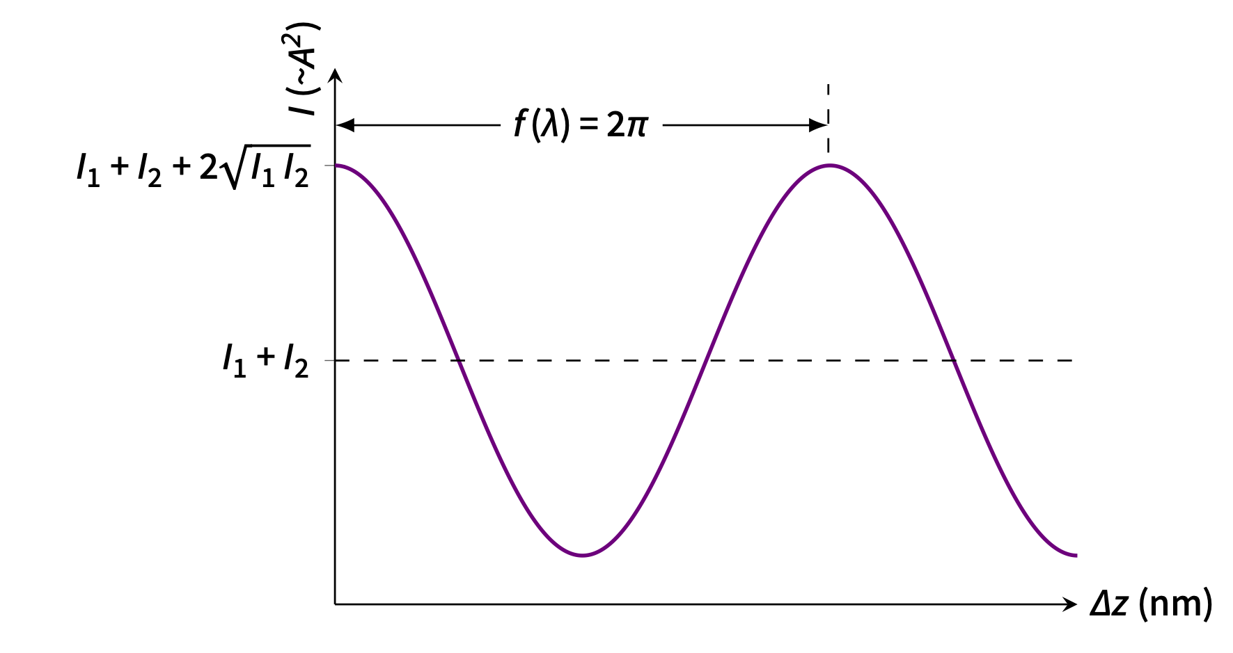
Optical detectors measure intensity, not the complex field directly ($I \propto |\psi|^2$): \[ I = \bigl|\left(A_1 e^{i\phi_1} + A_2 e^{i\phi_2}\right)\bigr|^2 = |A_1|^2 + |A_1|^2 + 2A_1A_2\cos(\Delta\varphi) . \]
Interference Intensity Relation
Expressing the individual beam intensities as $I_1 = A_1^2$ and $I_2 = A_2^2$ leads to
\[
I = I_1 + I_2 + 2\sqrt{I_1 I_2}\cos(\Delta\varphi) .
\]
The intensity therefore directly encodes the phase difference between the two beams.
Interferometry
Measurement Principle
Interferometry converts a change in optical path length into a measurable change in
intensity.
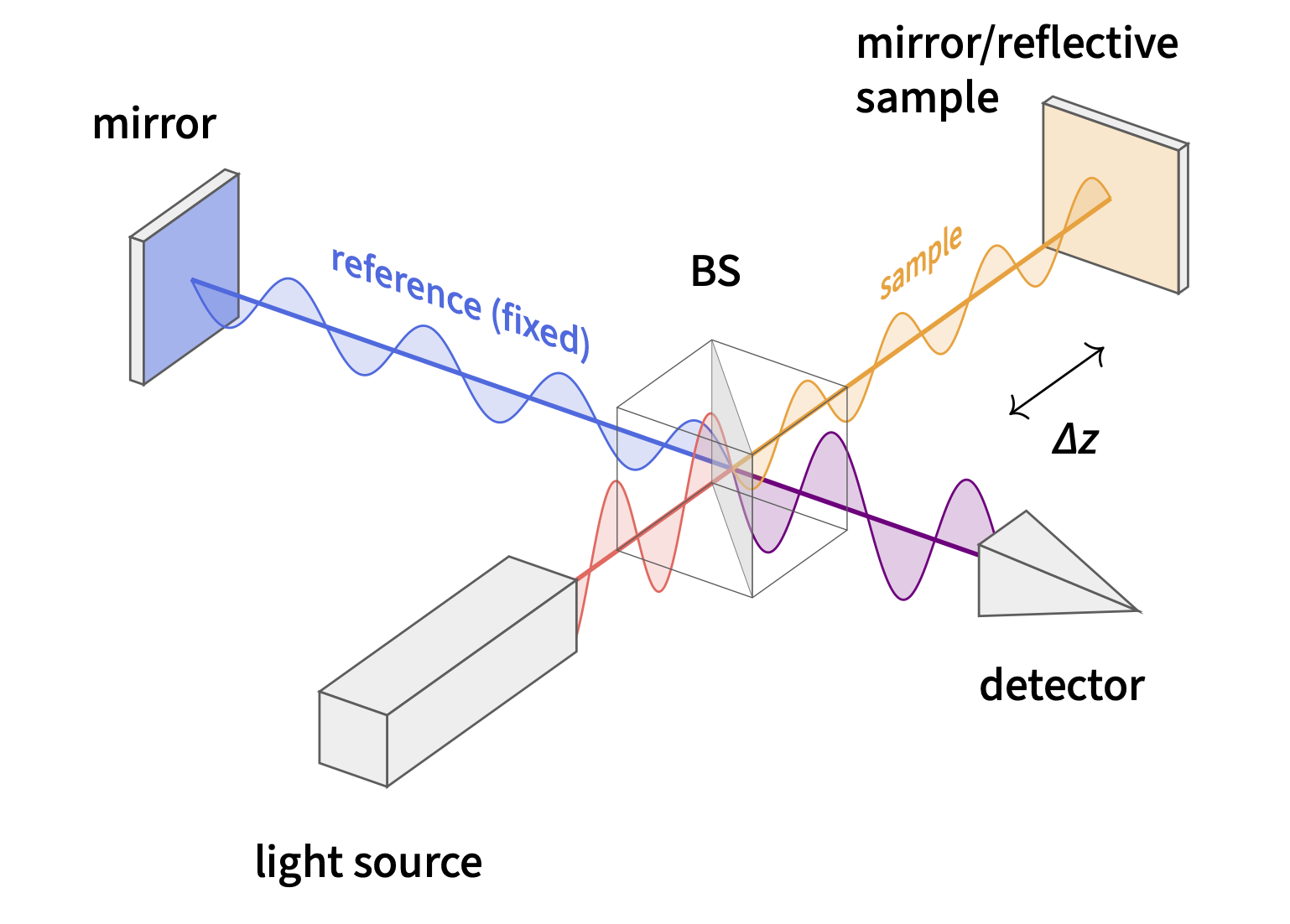
The fundamental principle involves splitting an incident light beam into two or more paths that traverse different optical path lengths before being recombined
In point detection, the interference signal is measured at a single location.
In full-field interferometry, the pattern is recorded simultaneously across an extended area using a camera.
Various interferometric configurations exist—including Michelson, Mach–Zehnder, and Fabry–Pérot interferometers—each offering specific advantages.
Michelson Type Interferometer (relevant to this work)
Light traverses the sample arm twice. A physical displacement \( \Delta z \) therefore produces a round-trip optical path difference of \(2\Delta z\). The corresponding phase shift is
\[
\Delta\varphi = \frac{4\pi}{\lambda}\Delta z.
\]
System Architecture
Key Idea
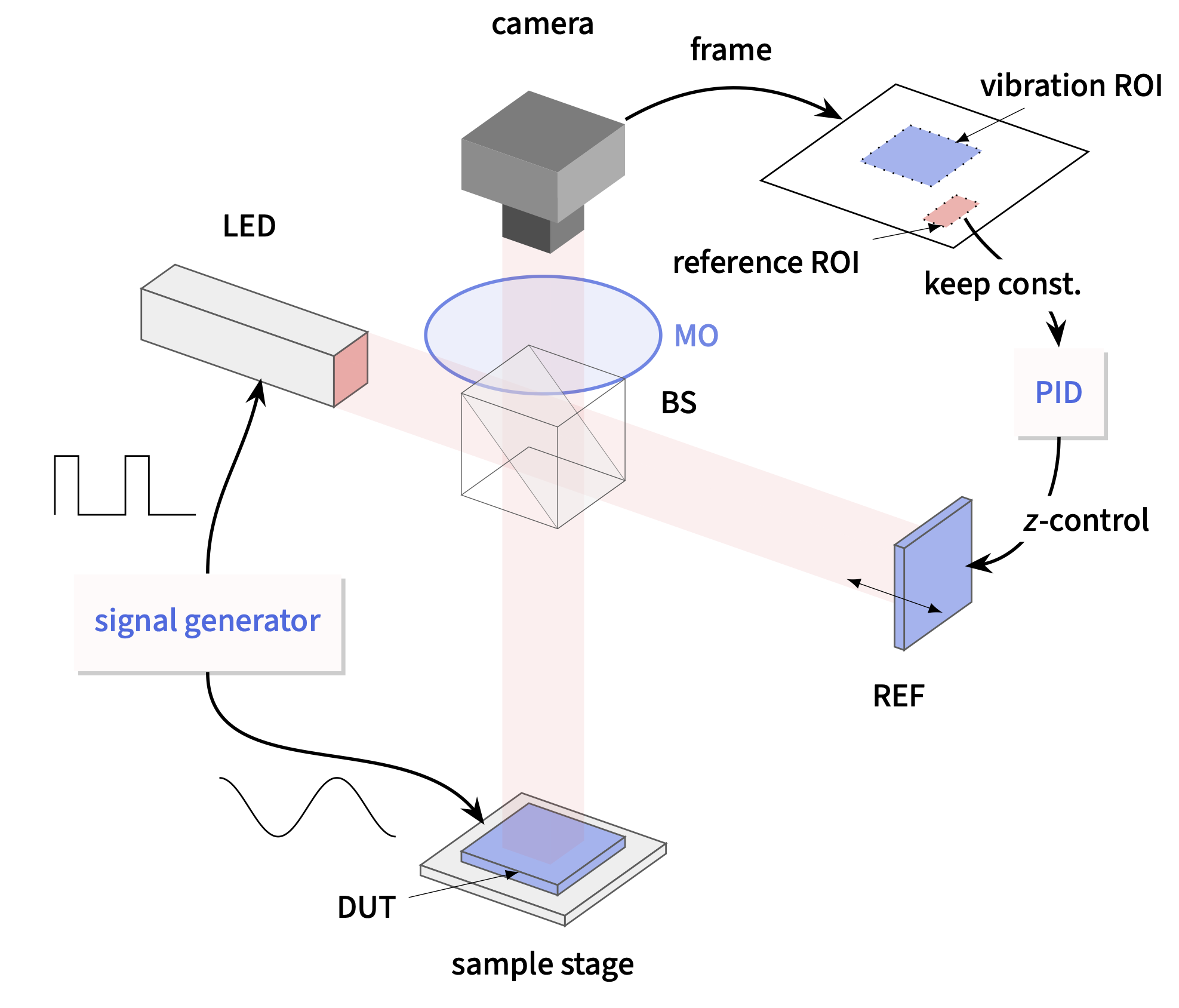
The system combines stroboscopic full-field Michelson interferometry with
software-controlled reference-arm stabilization.
Software-Based Stabilization
Continuous stabilization is required because the interferometer operating point can drift due to mechanical creep, thermal expansion, or external disturbances.
The system uses a software-based PID controller whose feedback is derived directly from the camera image.
Control Loop
- Measure mean image intensity inside non-vibrating reference ROI
- Compare with setpoint intensity (determined before the measurement)
- Compute PID correction
- Adjust reference mirror position
Constraint
The achievable closed-loop bandwidth is limited first by the camera frame rate.
At higher frame rates, acquisition and processing latency becomes the dominant bottleneck.
Operating Principle
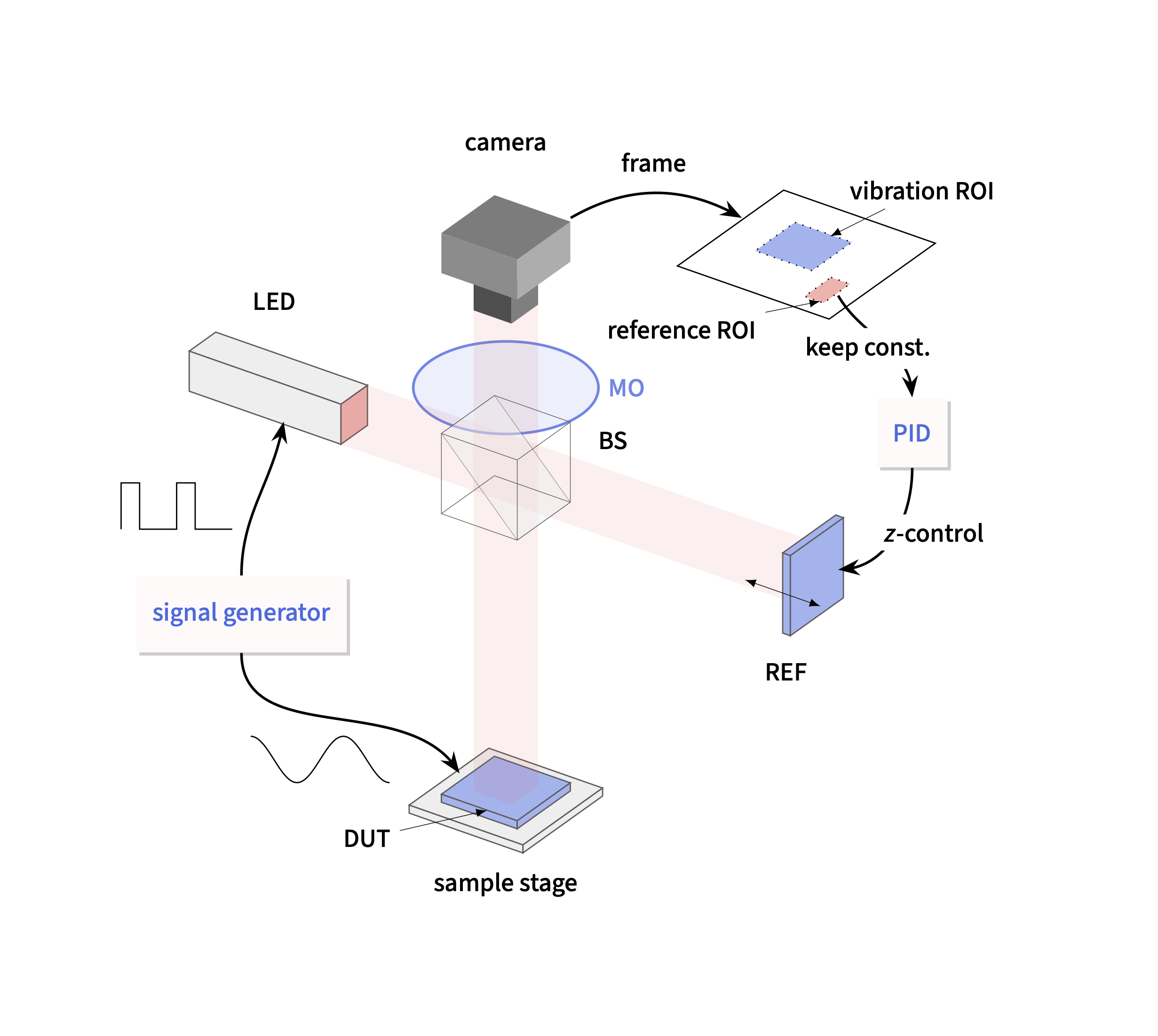
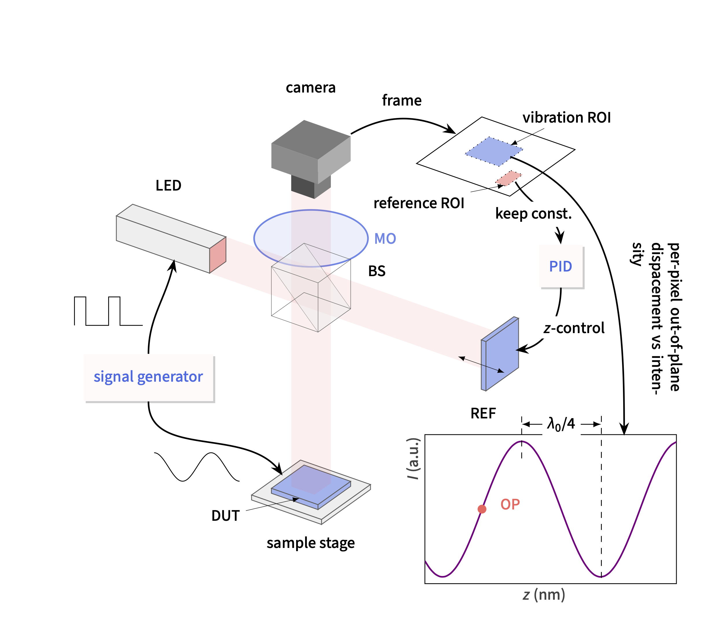
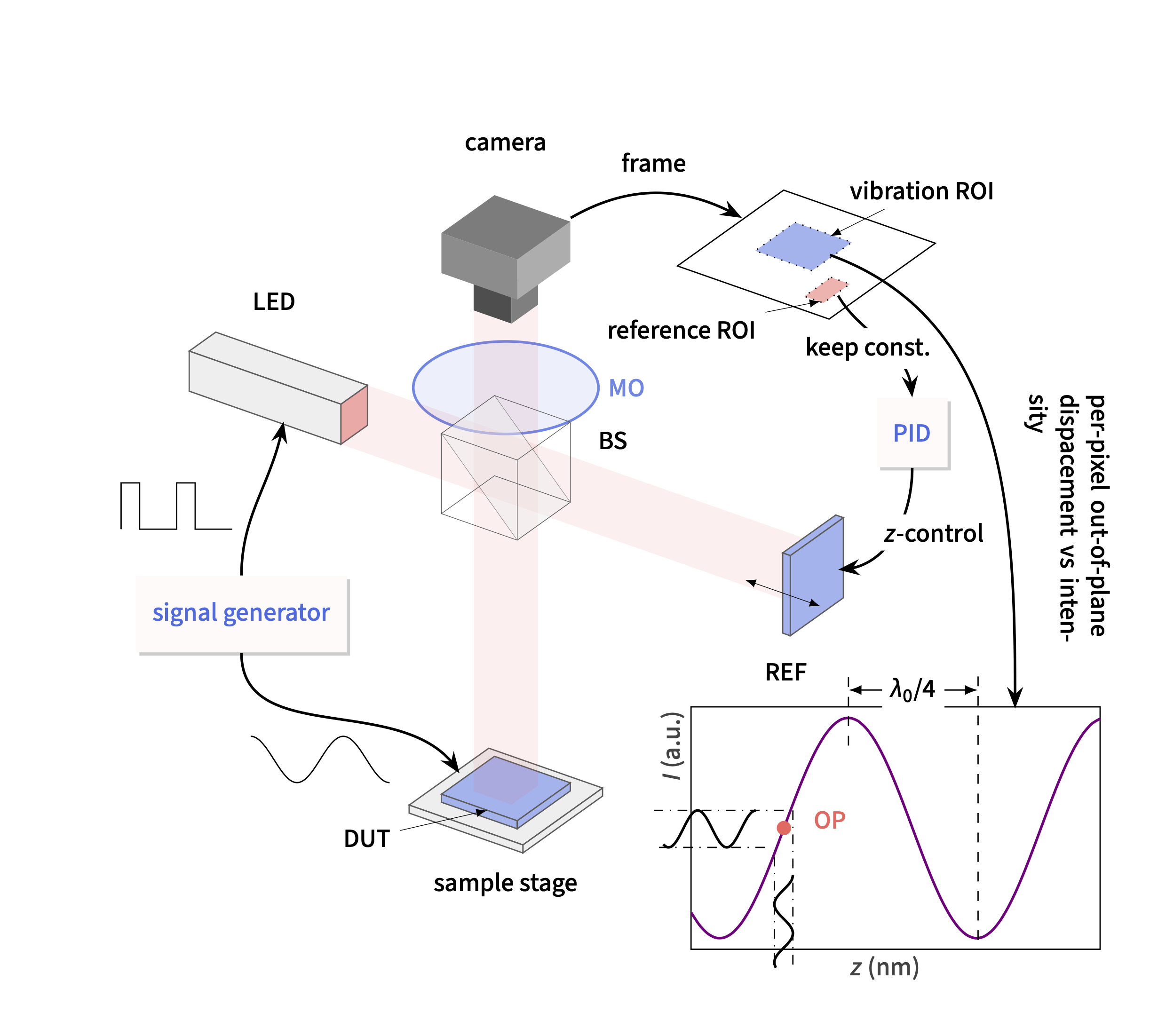
A surface displacement \(z(t)\) changes the optical path length in the sample arm and therefore modulates the interference phase.
\[
\Delta\varphi(t) = \Delta\varphi_0 + \frac{4\pi}{\lambda_0} z(t),
\]
where \( \Delta\varphi_0 \) is the static operating point phase.
Linearizing the interference signal around this operating point gives
\[
I(t) \approx I\!\left(\Delta\varphi_0\right)
+ \left.\frac{dI}{d\varphi}\right|_{\Delta\varphi_0}
\frac{4\pi}{\lambda_0} z(t).
\]
Key Idea
Near a fixed operating point, small displacements are encoded as linear intensity modulations.
Calibration and Operating-Point Selection
Practical Note
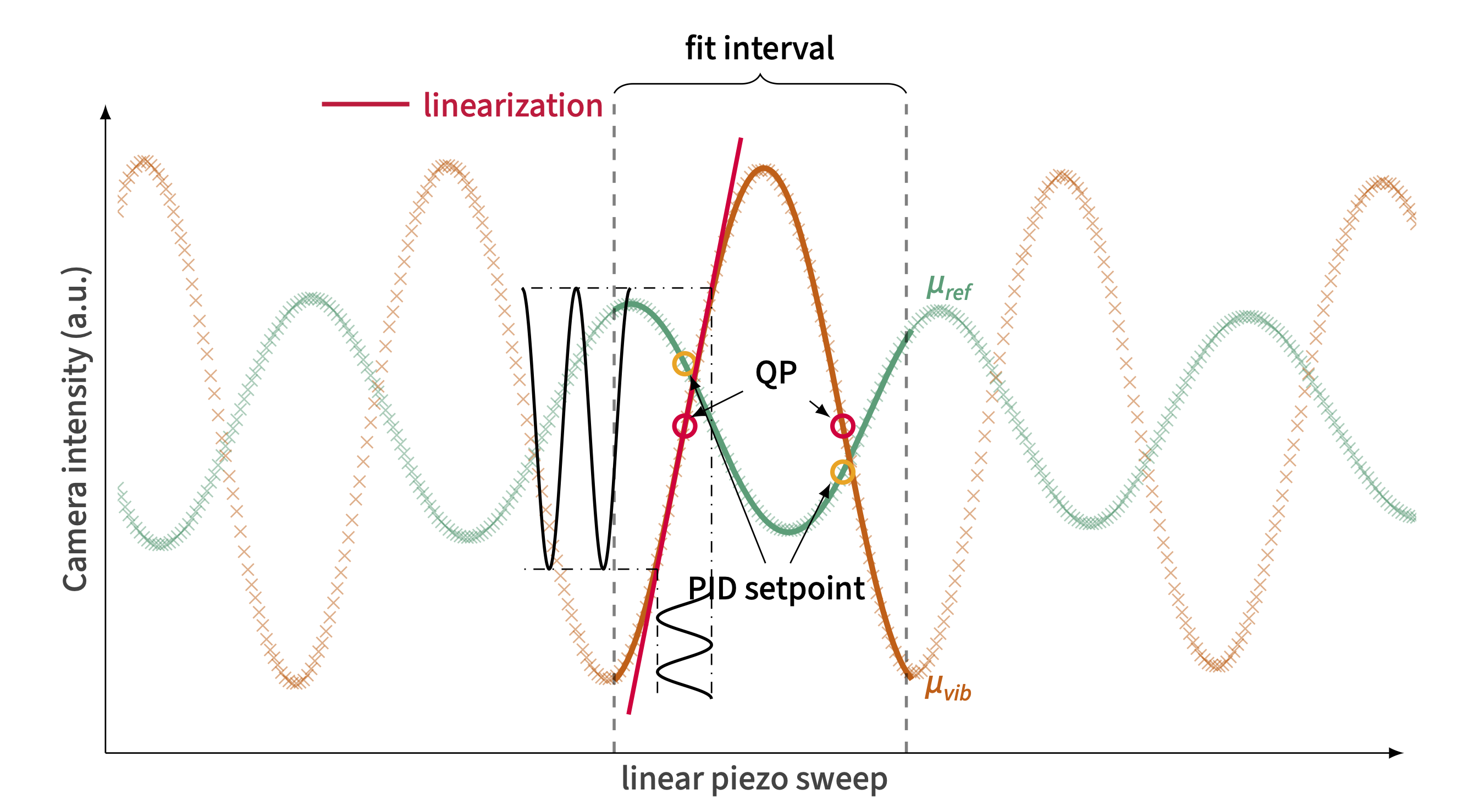
The PID setpoint must be sufficiently far from the extrema.
Otherwise drift may push the operating point beyond an extremum, the slope changes sign and the controller can relock to a neighboring quadrature point one fringe away.
The small-signal sensitivity depends on the operating point and is maximal at quadrature:
\[
\Delta\varphi_0 = \frac{(2m+1)\pi}{2}, \qquad m \in \mathbb{Z}.
\]
A piezo sweep of the reference mirror is used to record the mean intensities in a reference ROI and a vibration ROI.
A difference in surface height between these ROIs results in phase-shifted intensity curves.
By fitting sinusoidal models to both curves the optimal measurement operating points are identified and provide the corresponding PID setpoints.
Purpose of Calibration
Calibration identifies operating points with high sensitivity and maps them to stabilization setpoints for
closed-loop operation.
Pixel-Wise Sensitivity and Displacement Mapping
Measurement Modalities
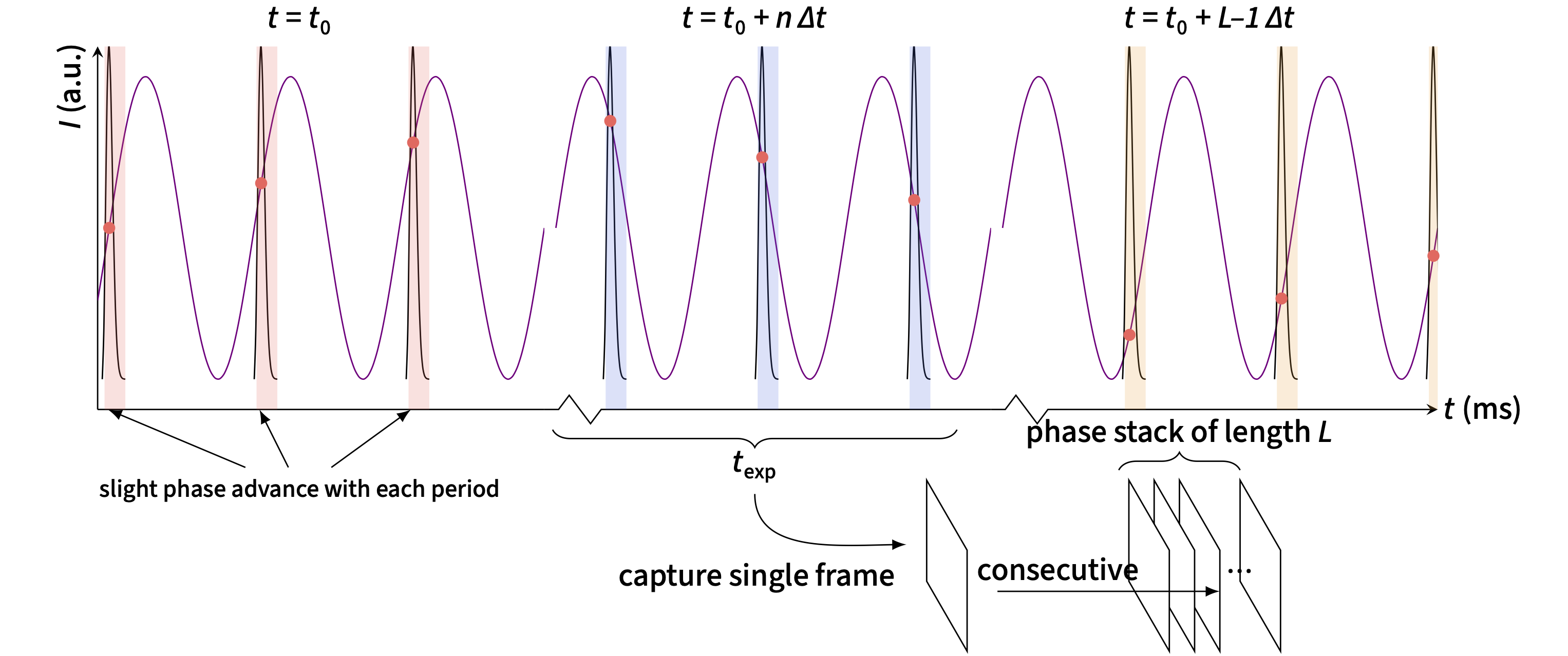
Continuous with Shifted Frequencies
The DUT and LED are driven at slightly different frequencies,
\[
f_{\mathrm{DUT}} = f_{\mathrm{LED}} + \Delta f.
\]
The relative phase then evolves at the beat frequency \( \Delta f \), so the vibration appears in
apparent slow motion with synthetic period
\[
T_{\mathrm{beat}} = \frac{1}{\Delta f}.
\]
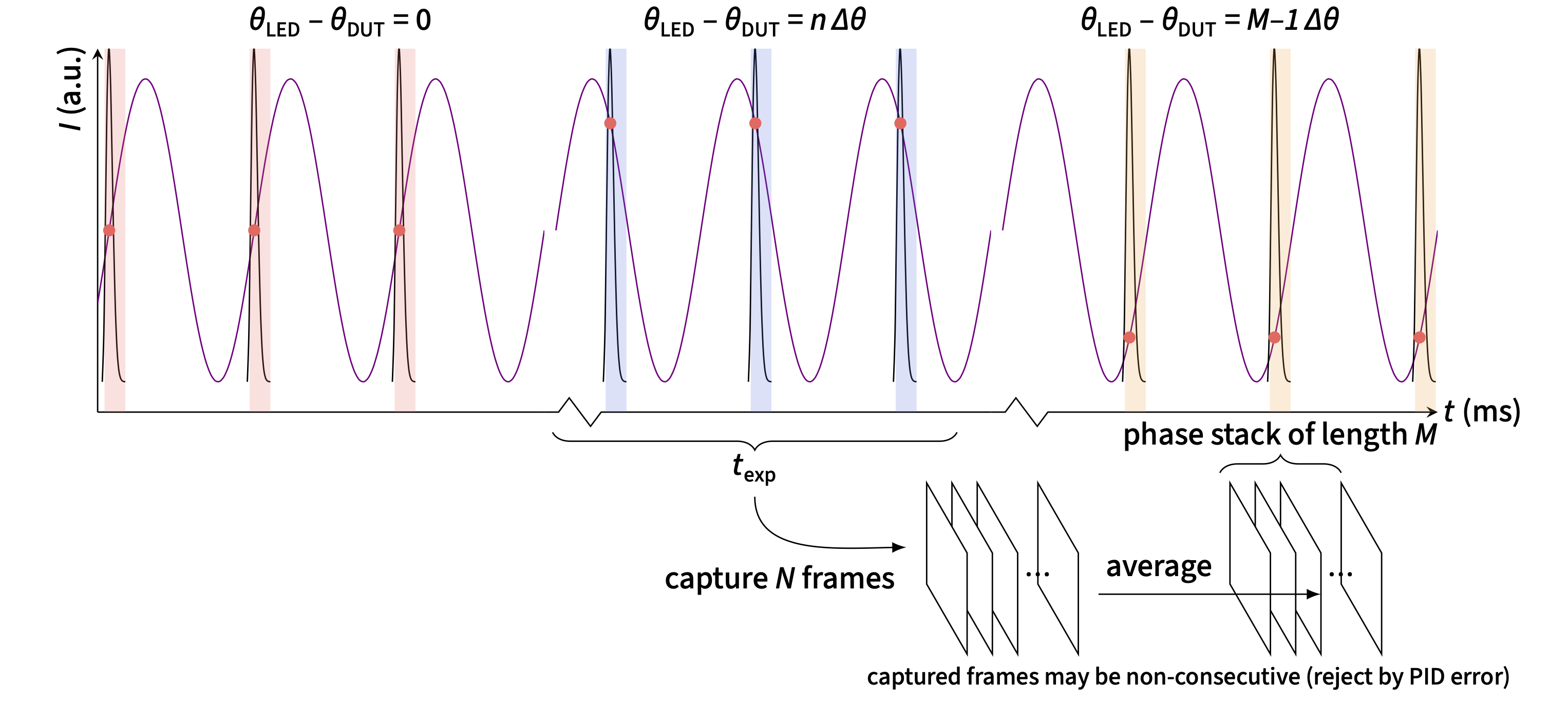
Phase Stepping with Averaging
The LED and DUT are driven at the same frequency,
\[
f_{\mathrm{LED}} = f_{\mathrm{DUT}}.
\]
A full vibration cycle is reconstructed by stepping the relative phase in
\[
\Delta\theta = \frac{2\pi}{M}
\]
increments and averaging \(N\) frames per step, which improves SNR by approximately
\( \sqrt{N} \).
Use Case
Shifted-frequency acquisition is useful for rapid frequency sweeps and immediate visual feedback.
For quantitative measurements, the preferred modality is
phase stepping with averaging.
The Complete Measurement Workflow
Amplitude and Phase Extraction Procedure
Displacement Reconstruction
Sample Introduction

Practical Measurement Constraint
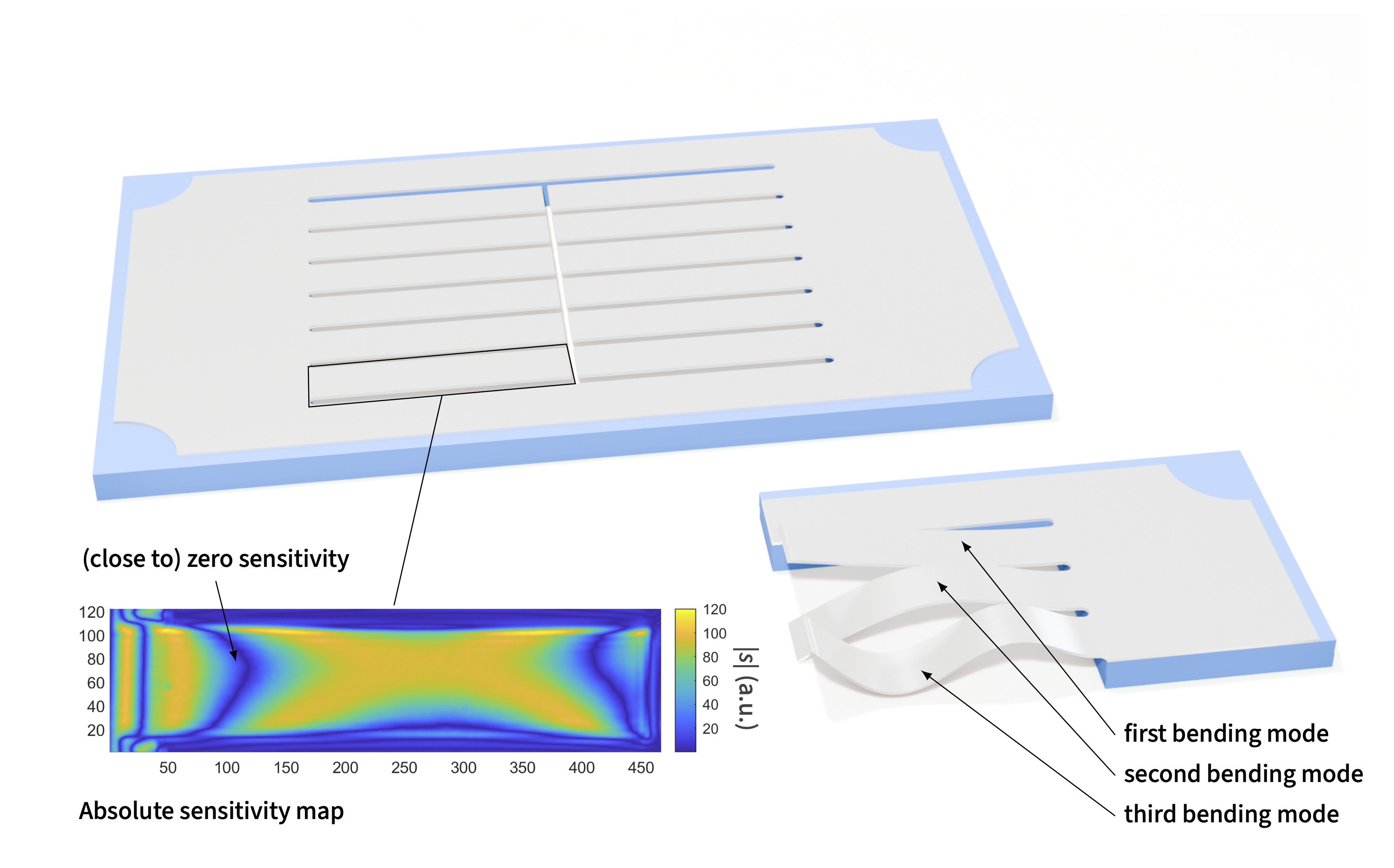
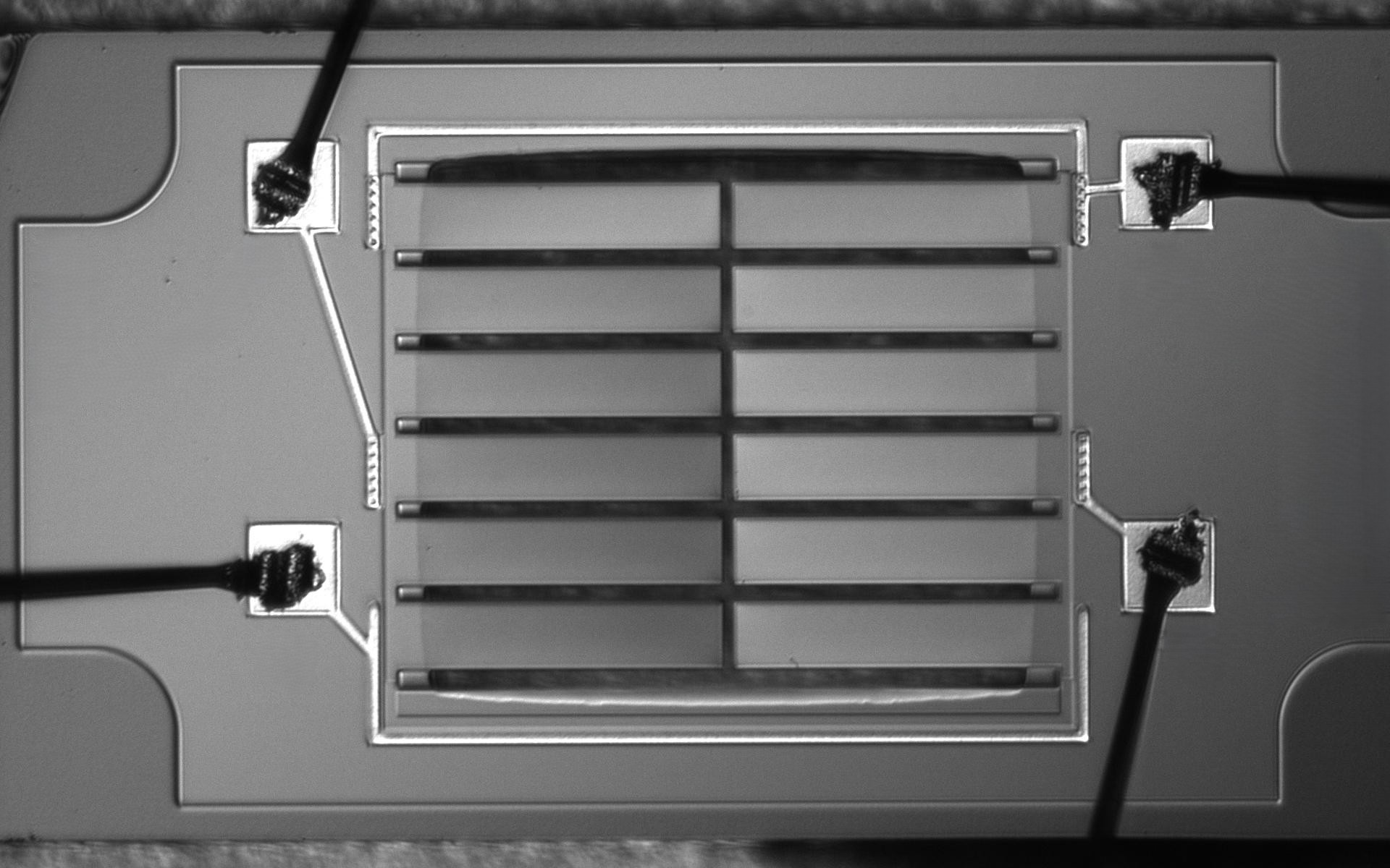
Interferometric sensitivity is best on locally flat surfaces. Because some cantilevers exhibit static curvature or tilt,
a beam with minimal out-of-plane deformation was selected and aligned as closely as possible to the optical axis.
Sample Features
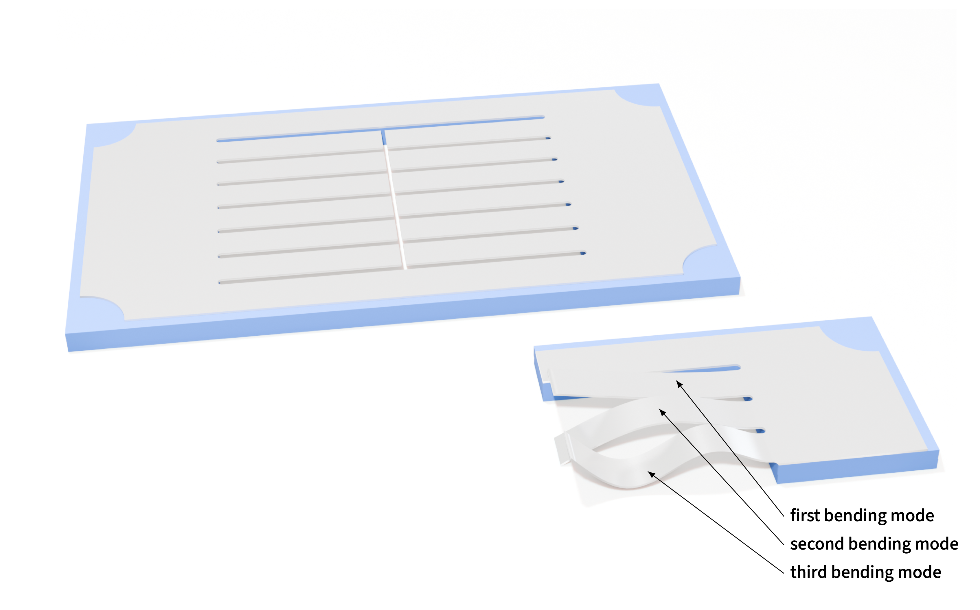
- Piezoelectrically actuated cantilever array on a single chip
- Nominally identical beam geometry and material stack
- Released by anisotropic backside etching
- Spatial sampling: \(\sim 1\,\mathrm{µm}\) per pixel
- Typical beam size in the image: \(\sim 400 \times 80\) px
- All beams driven simultaneously via the integrated piezoelectric layer
Frequency Response Measurement
Interpretation
The increase in \(Q\) with mode order is qualitatively consistent with reduced anchor-loss contribution
and weaker effective air damping at higher frequencies.
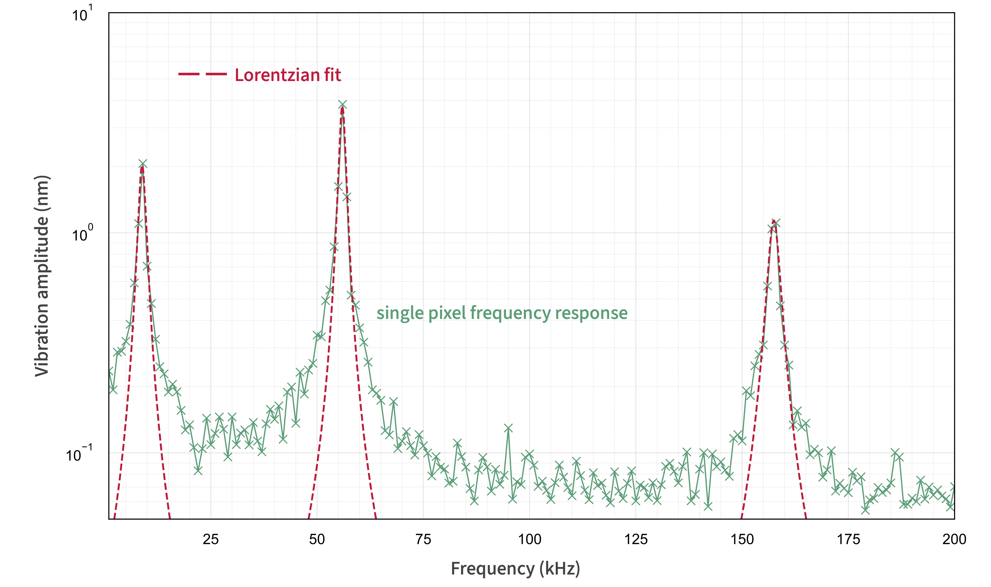
A coarse frequency sweep from \(1\) to \(200\,\mathrm{kHz}\) in \(1\,\mathrm{kHz}\) steps was performed using \(M=18\) phase steps, \(n_p=4\) periods, and \(N=4\) averaged frames per step.
A pixel in the central span of the beam, \((x,y)=(200,60)\), was monitored to generate a representative response curve.
Three prominent resonance peaks were identified and refined using Lorentzian fits. \[ A(f) \;=\; A_0\,\frac{1}{\sqrt{1 + \left(\frac{2Q}{f_n}\right)^2 (f-f_n)^2}}, \]
Extracted Resonances
- \(f_1 \approx 8.8\,\mathrm{kHz}, \qquad Q_1 \approx 4\)
- \(f_2 \approx 55.9\,\mathrm{kHz}, \qquad Q_1 \approx 30\)
- \(f_3 \approx 157.5\,\mathrm{kHz}, \qquad Q_1 \approx 48\)
Validation Against Euler–Bernoulli Beam Theory
Validation Assessment
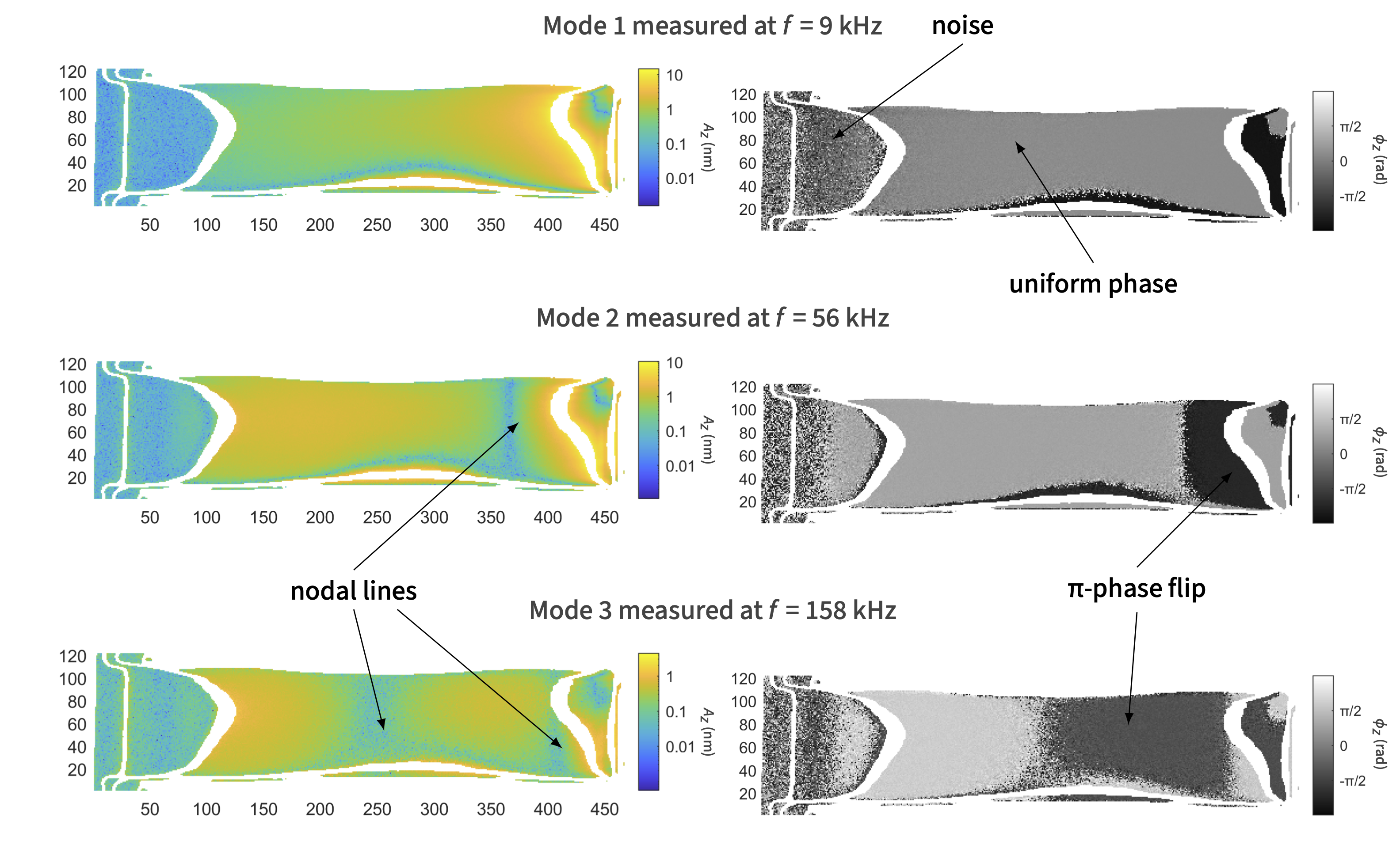
The measured resonance frequencies agree well with Euler–Bernoulli beam theory.
In addition, the phase maps exhibit the expected nodal structure of the first three clamped–free bending modes.
To assess physical consistency, the measured resonances are compared with the Euler–Bernoulli model for a uniform clamped–free beam:
\[ f_n = \frac{\beta_n^2}{2\pi L^2}\sqrt{\frac{EI}{\rho A}}, \] with \(\beta_1=1.875,\;\beta_2=4.694,\;\beta_3=7.855,\ldots \)
Frequency ratios eliminate dependence on unknown composite parameters:
\[
\frac{f_n}{f_1}=\left(\frac{\beta_n}{\beta_1}\right)^2,
\qquad
\frac{f_2}{f_1}\approx 6.27,
\qquad
\frac{f_3}{f_1}\approx 17.55.\\
\]
Validation Results
- \(f_2/f_1 = 6.3, \qquad \varepsilon = 1.0\%\)
- \(f_3/f_1 = 17.8, \qquad \varepsilon = 1.6\%\)
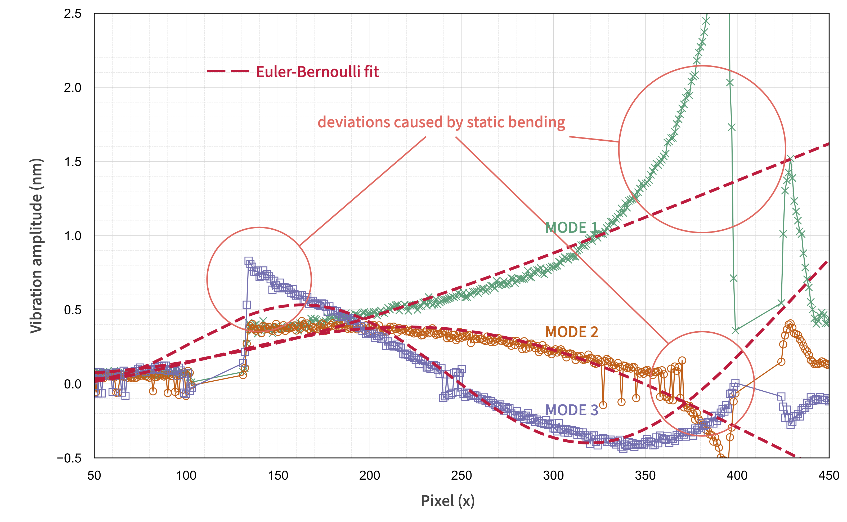
Mode-Shape Fits Along the Beam Centerline
Fit Assessment
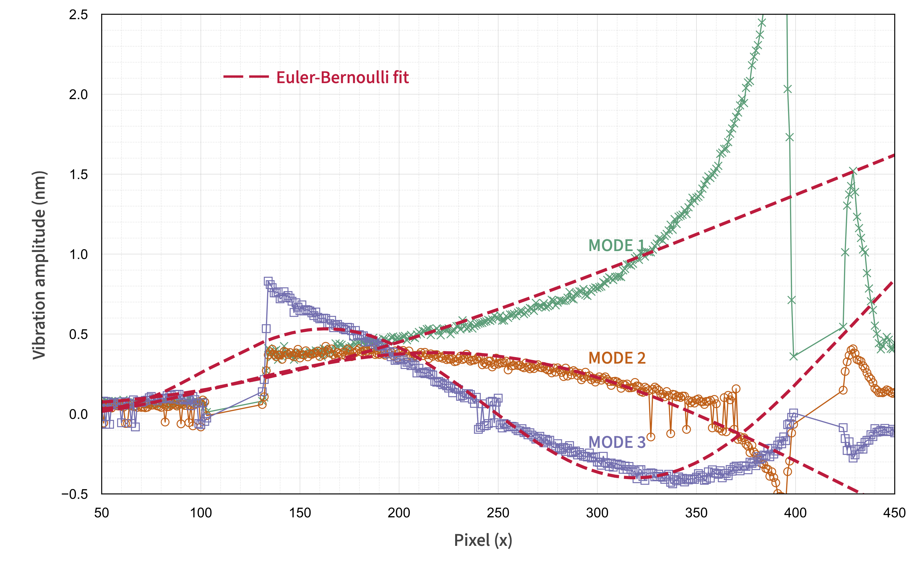
Modes 1 and 2 yield mutually consistent fit parameters, while mode 3 deviates more strongly.
Nevertheless, the inferred beam lengths remain close to the nominal \(\sim 400\) px scale,
and the analytical shapes agree well with the measured profiles outside excluded regions.
For a more quantitative comparison, the measured centerline displacement profile is fit to the analytical clamped–free Euler–Bernoulli beam shape.
\[ \begin{align} &\phi_n(x)\\ &=A_n\Bigl[\cosh(\beta_n x)-\cos(\beta_n x) -\eta_n\bigl(\sinh(\beta_n x)-\sin(\beta_n x)\bigr)\Bigr], \end{align} \] with \[ \eta_n= \frac{\cosh(\beta_n L)+\cos(\beta_n L)} {\sinh(\beta_n L)+\sin(\beta_n L)}. \]
To account for uncertainty in clamp position and pixel origin, horizontal and vertical offsets are included as fit parameters.
Regions with outliers or low sensitivity are excluded from the fit.
Fit Parameter Results
| $n$ | $A_n$ (arb.) | $L$ (px) | $x_0$ (px) | $y_0$ (arb.) |
|---|---|---|---|---|
| 1 | 0.78 | 430.0 | -17.0 | 0.06 |
| 2 | 0.27 | 423.0 | -19.5 | -0.01 |
| 3 | 0.33 | 388.8 | 10.1 | 0.03 |
Noise Analysis
Interpretation
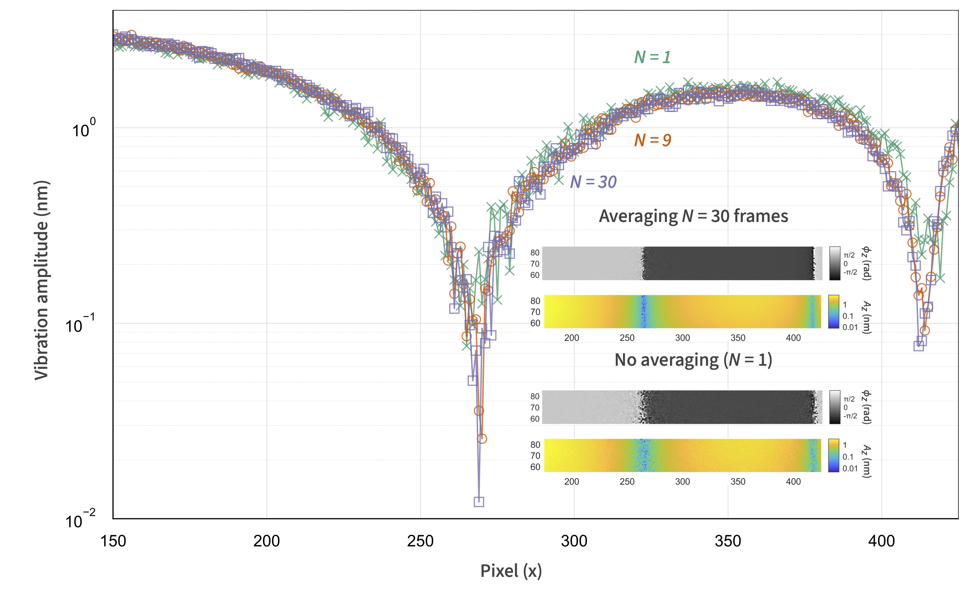
Ideally, averaging improves SNR by approximately \( \sqrt{N} \).
From \(N=9\) to \(N=30\), this would predict an improvement factor of
\[
\sqrt{30/9} \approx 1.8.
\]
The weaker observed gain suggests that slow lateral drift becomes the dominant limitation.
A direct noise-floor measurement would require strict pixel correspondence across repeated acquisitions, which is currently limited by uncorrected lateral drift.
Measurement Parameters
As a qualitative alternative, measurements were compared at \(f=158\,\mathrm{kHz}\) for
averaged frames per phase step, with all other parameters held fixed.
- \(N=1\)
- \(N=9\)
- \(N=30\)
In the third bending mode, the profile line at \(y=70\) shows that averaging produces cleaner nodal transitions and deeper minima. The improvement from \(N=9\) to \(N=30\), however, is only marginal.
Practical Noise Floor
The smallest detectable out-of-plane vibration amplitude is estimated to be on the order of
\[
\sim 200\,\mathrm{pm}.
\]
Limitations and Future Directions
Any Questions?